 Hoy, vamos a conversar un poco sobre R y Rstudio un software GPL desarrollado en Nueva Zelanda, para realizar operaciones de minería de texto, Econometria, Estadísticas Avanzadas, de la mano de les traigo unos snipets de código bastante buenos que les ayudaran a comprender y usar R, primero que todo para poder comenzar con R debemos tener el software necesario, para ello descargamos desde aqui el lenguaje y Rstudio desde aca, que es el IDE de programación.
R, es un potente software que se puede adherir a una basta fuente de datos, herramientas como SAP_HANA, Tableau – Pentaho – Oracle y otras mas, estos productos han incorporado R en su plataforma ademas funciona en cualquier sistema operativo. Durante la sesión de trabajo con R pudimos extraer algunos Tips los cuales les detallo a continuación:
El debbuger de R es bastante bueno y a la hora de un error en el código, el mismo arroja información compresible como por ejemplo:
> solve(M)
Error in solve.default(M) : ‘a’ (4 x 5) must be square
- Ctrl – L Limpia la pantalla de la consola.
- Historial de ejecución (Flechas de dirección).
- Ejecución rápida de bloques de código (Selección y Ctrl – R)
- Tiene biblioteca de consulta para las funciones integradas (> help(“order”).
- Dispone de la función “apropos” su utilidad radica en ubicar en la linea de nombre y descripción de los paquetes implementados en R el patrón de búsqueda indicado, esto te ayudaría a encontrar una función que no conoces para cumplir una determinada tarea.
- Si faltara un paquete que no consigues puedes ajustar la linea del servidor CRAN de la siguiente forma:
install.packages(“RJSONIO”, repos = “http://www.omegahat.org/R”, type=”source”)
- De lo contrario aplica la siguiente linea:
install.packages(“ggplot2”, dependencies=TRUE)
Y sin mas preámbulos acá les dejo este bloque de código R que trae varios ejemplos y esta bien documentado:
############################################################
# Establecer área de trabajo
############################################################
setwd(“C:/ruta/ruta/ruta”) #se crea el área de trabajo
############################################################
# Simples Manipulaciones
############################################################
x = c(1, 2.5, 3.8, 4) # Creación de vector
y = 1:20 # Genera una secuencia de números del 1 al 20
w = seq(-1,1,by=0.1); w[5]
z = w^2 + 1 # Operaciones básicas con *, +, -, / y ^
# Crear Matrices
M = array(1:20, dim=c(4,5))
N = matrix(1:20, nrow=4,ncol=5)
M[2,4] # Ver la posición 2, 4 de la matriz
N[1:2,1:3] # Sub-matriz
P = M%*%t(N); M+N # Producto y suma de matrices
P1 = cbind(M,N); P2=rbind(M,N) #Matrices combinadas
dim(M); nrow(M); ncol(M) # Dimensión de una Matriz
# Inversa de una matriz nxn
C=matrix(c(2,3,3,0),nrow=2,ncol=2)
solve(C)
############################################################
# Listas
############################################################
Lst[[4]]
# Autovales y autovectores
ev = eigen(C) # Resultado obtenido es una lista
ev$values
ev$vectors
############################################################
#Funciones Elementales (log, exp, sin, cos, tan, sqrt,mean, max, min, length, etc)
#############################################################
x=rnorm(10, mean = 0, sd = 1)
sum((x-mean(x))^2)/(length(x)-1)
#############################################################
# Consultas lógicas (==, !=, >,<,>=,<=, &, |, ! )
#############################################################
x>=0.5
y=3
y!=3 & y>0
#############################################################
# Datos faltantes (NA)
#############################################################
z=c(1:3,NA)
#############################################################
# Leer y guardar datos
#############################################################
head(data)
names(data)[1]=”City”
write.csv(data,file=”USArrests.csv”, row.names=FALSE) # Otra write.table
#############################################################
# Sentencias de control
#############################################################
# Condicionales (if)
if (y!=3){
print(“y es distinto de 3”)
} else{
print(“y es igual a 3”)
}
#Repetitivas (for, while)
x=c(“carne”,”hoja”,”camión”, “dinosaurio”,”hoja”,4,”perro”)
count=0
for(i in 1:length(x)){
if(x[i]==”hoja”){
count=count+1
}
}
count
count=0;k=0
while(k<length(x)){
k=k+1
if(x[k]==”hoja”){
count=count+1
}
}
# o mas simple
sum(x==”hoja”)
#############################################################
# Crear funciones
#############################################################
bartop=function(x,n,column_name){
i=which(colnames(data)==column_name)
title= paste(column_name,”Rate”,sep=” “)
data=x[rev(order(x[,i])),]
barplot(data[1:n,i], names.arg = data$City[1:n], las = 2, ylab = column_name, main = title)
}
bartop(data,10,”Murder”)
pdf(“prueba_hist.pdf”) #Guardar la salida en pdf
bartop(data,10,”Murder”)
dev.off() # cierro la ventana donde se escribirá el histograma al archivo
#############################################################
# Instalar paquetes
#############################################################
installed.packages() # Vemos que paquetes hay instalados
install.packages(“stringi”, dependencies=TRUE) # Paquete para procesar texto.
library(stringi)
# Encontrar una o varias palabras
texto=”R es un software estadístico, super poderoso.”
stri_detect_fixed(texto, “estadístico”)
words=c(“poderoso”,”super”)
stri_detect_fixed(texto, words)
stri_split_fixed(texto,” “)
#############################################################
# Retomemos las funciones repetitivas apply, lapply, sapply.
#############################################################
apply(data[,2:5],1,mean) # Se obtiene la media de cada fila.
apply(data[,2:5],2,mean) # Se obtiene la media de cada columna.
sapply(1:3, function(x) x^2) # Salida vector.
sapply(1:3, function(x) x^2, simplify=F) # Salida es una lista.
sapply(1:length(palabras), function(i,x){str_split_fixed(x[i],” “)},palabras) #Obtenemos una lista
lapply(1:3, function(x) x^2)
#############################################################
# Gráficos
#############################################################
#Graficos de Rbase
par(mfrow=c(2,2),bg=”white”)
attach(data)
plot(Murder,Assault, col=”red”,main=”Murder vs Assault”, cex=0.5, pch=19)
text(Murder, Assault, labels = City, cex= 0.7, adj = c(0.5, 1))
barplot(Murder, names.arg = City, las = 2, ylab = “# Murder per 100,000″, main=”Murder Rate”)
slice=data[rev(order(data$UrbanPop)),]
pie(slice[1:5,2],labels = slice[1:5,1], col=rainbow(length(slice[1:5,2])), radius=3,
main=”Pie of Top UrbanPop”)
#GrÃficos de paquetes
install.packages(“ggplot2”, dependencies=TRUE)
library(“ggplot2”)
weather=read.csv(“weather_2014.csv”,header=TRUE,sep=”;”) # Datos del clima en Porto.
first.day=as.date(“2014-01-01”)
weather$date=first.day + weather$day.count – 1
ggplot(weather, aes(x = date,y = ave.temp)) + geom_point(aes(color = ave.temp)) +
scale_colour_gradient2(low = “blue”, mid = “green” , high = “red”, midpoint = 16) +
geom_smooth(color = “red”,size = 1) + scale_y_continuous(limits = c(5,30), breaks = seq(5,30,5)) +
ggtitle (“Daily average temperature”) + xlab(“Date”) + ylab (“Average Temperature ( ºC )”)
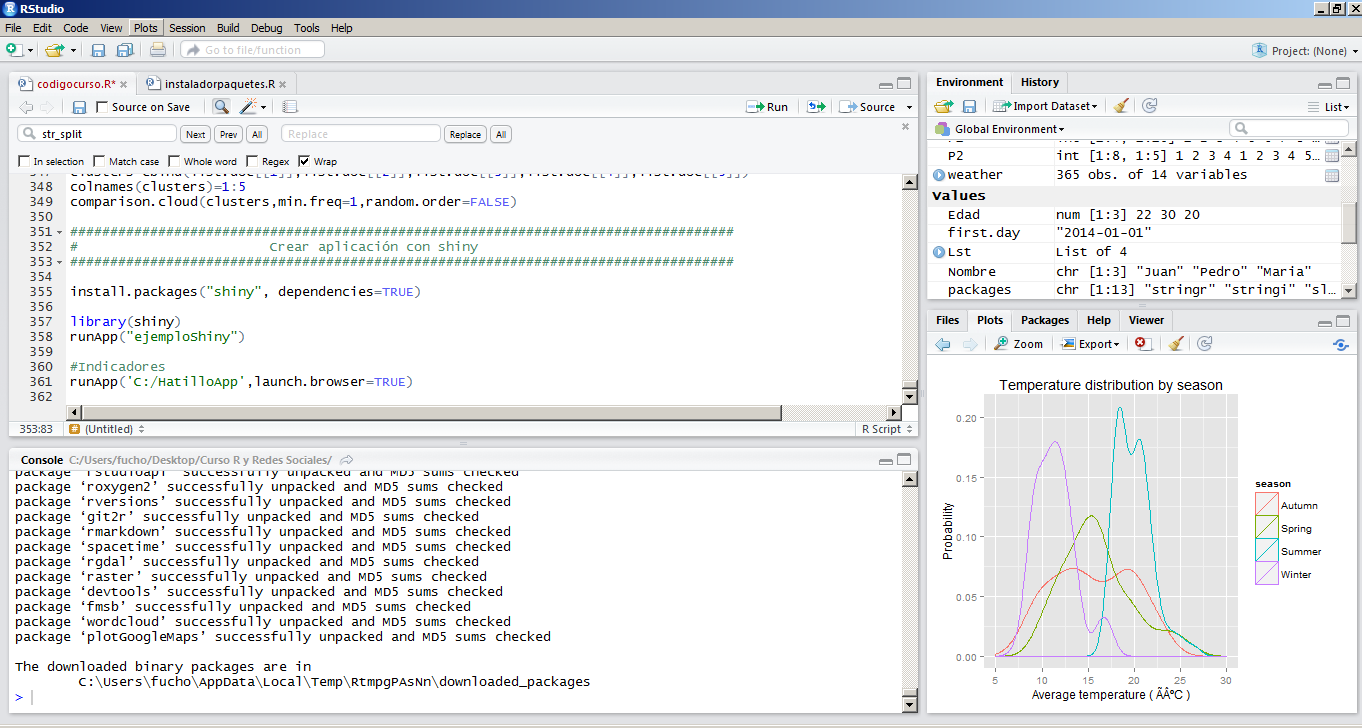
ggplot(weather,aes(x = ave.temp, colour = season)) + geom_density() +
scale_x_continuous(limits = c(5,30), breaks = seq(5,30,5)) +
ggtitle (“Temperature distribution by season”) + xlab(“Average temperature ( ºC )”) +
ylab (“Probability”)
#############################################################
# Obtener datos twitter
#############################################################
install.packages(“twitteR”, dependencies=TRUE)
library(“twitteR”)
apiKey=”XN4EWAv67kQkdxaeGaUikc4Zk”
apiSecret=”flc6kQ25yyX38TpdgsoXhVuELWINRYM6rMOYhxV3CVE03dHn1d”
access_token=”143571664-0dhE1qtuheKJAaNAERNtQFJVIBg4Ckc41VA6ObWo”
access_token_secret=”HpTTpqLyVanOBn7lDQpidwYPH2acO0E2rcvnQcD0Pr7ro”
my_oauth=setup_twitter_oauth(apiKey,apiSecret,access_token,access_token_secret)
tweets=searchTwitter(“Venezuela”, n=500,lang=”es”)
tweets=twListToDF(tweets) # Extraer información extra a un data.frame
# Obtener el timeline de un usuario
timeline=userTimeline(“MatrixDataLabs”,n=1000)
timeline=twListToDF(timeline)
# Amigos y Seguidores
mdl=getUser(“MatrixDataLabs”)
following=mdl$getFriends()
following=twListToDF(following) # Obtenemos un perfil completo de cada seguidor
follower=mdl$getFollowers()
follower=twListToDF(follower)
#############################################################
# Procesamiento de texto
#############################################################
# Limpieza
tweets.text=tweets[,1]
#Borrar caracteres especiales
tweets.text=gsub(“[^[:print:]]“, ” “, tweets.text)
# Borrar enlaces
tweets.text=gsub(“http[^ ]+”, ” “, tweets.text)
#Convertir todo el texto en minusculas.
tweets.text=tolower(tweets.text)
#Reemplazar patron (???rt???)
tweets.text=gsub(” rt “, ” “, tweets.text)
#Borrar puntuación
tweets.text=gsub(“(?!@)(?!#)[[:punct:]]”, ” “, tweets.text, perl=TRUE)
#Borrar varios espacios en blanco seguidos
tweets.text=gsub(“[ |\t]{6,7}”, ” “, tweets.text)
tweets.text=gsub(“[ |\t]{4,5}”, ” “, tweets.text)
tweets.text=gsub(“[ |\t]{2,3}”, ” “, tweets.text)
# Remover espacios en blanco al comienzo
tweets.text=gsub(“^ “, “”, tweets.text)
# Remover espacios en blanco al final
tweets.text=gsub(” $”, “”, tweets.text)
# Remover números
tweets.text=gsub(“\\d”, ” “, tweets.text)
install.packages(“tm”, dependencies=TRUE)
install.packages(“slam”, dependencies=TRUE)
library(tm)
library(slam)
#Borrar algunas palabras
borrar=read.csv(“C:/Users/ruta/ruta/articulos.csv”, fileEncoding=”latin1″)
borrar=as.character(borrar[,1])
tweets.text=removeWords(tweets.text,borrar)
#create corpus
tweets.text.corpus=Corpus(VectorSource(tweets.text)) #Obtiene la metadata de la colección de los documentos.
matrix.corpus=TermDocumentMatrix(tweets.text.corpus, control = list(minWordLength = 1))
inspect(matrix.corpus[1:10,1:10])
# Frecuencia de palabras
findFreqTerms(matrix.corpus, lowfreq=10)
# which words are associated with “inflación”
findAssocs(matrix.corpus, ‘inflación’, 0.30)
matrix.corpus2=rollup(matrix.corpus, 2, na.rm=TRUE, FUN = sum) # Hace una agregación de los datos.
m=as.matrix(matrix.corpus2)
# compute the frequency of words
v=sort(rowSums(m), decreasing=TRUE)
myNames=names(v)
d=data.frame(word=myNames, freq=v)
install.packages(“wordcloud”, dependencies=TRUE)
library(wordcloud)
pal=brewer.pal(8,”Dark2″) # Palletes of colors.
wordcloud(d$word, d$freq, min.freq=10, scale=c(4,0.5),colors=pal,random.order=F)
#############################################################
# Análisis de sentimientos.
#############################################################
score.sentiment = function(tweets.text, pos, neg){
borrar=read.csv(“C:/Users/ruta/ruta/Curso R y Redes Sociales/articulos.csv”, fileEncoding=”latin1″)
borrar=as.character(borrar[,1])
neg=read.csv(“C:/Users/ruta/Curso R y Redes Sociales/negative_words.csv”, fileEncoding=”latin1″)
pos=read.csv(“C:/Users/ruta/Curso R y Redes Sociales/positive_words.csv”, fileEncoding=”latin1″)
neg=as.character(neg[,1])
pos=as.character(pos[,1])
tweets.text=gsub(“[^[:print:]]“, ” “, tweets.text)
tweets.text=gsub(“[[:punct:]]”, ” “, tweets.text)
tweets.text=tolower(tweets.text)
tweets.text=gsub(“rt”, ” “, tweets.text)
tweets.text=gsub(“@\\w+”, ” “, tweets.text)
tweets.text=gsub(“http.+”, ” “, tweets.text)
tweets.text=gsub(“[ |\t]{6,7}”, ” “, tweets.text)
tweets.text=gsub(“[ |\t]{4,5}”, ” “, tweets.text)
tweets.text=gsub(“[ |\t]{2,3}”, ” “, tweets.text)
tweets.text=removeWords(tweets.text,borrar)
scores = sapply(tweets.text, function(tweets.text, pos, neg) {
pos.matches = stri_detect_fixed(tweets.text, pos)
neg.matches = stri_detect_fixed(tweets.text, neg)
score = sum(pos.matches) – sum(neg.matches)
return(score)
}, pos, neg)
scores.df = data.frame(score=scores, text=tweets.text)
return(scores.df)
}
out1=score.sentiment(tweets.hatillo[,1], pos, neg)
sent=vector(length=nrow(out1))
sent[which(out1$score<=-1)]=”negative”
sent[which(out1$score>=1)]=”positive”
sent[which(out1$score==0)]=”neutro”
out1=cbind(out1,sent)
tweets=data.frame(tweets,”Sentimiento”=out1[,3])
#Clusters de documentos
doc.matrix=t(as.matrix(matrix.corpus))
wss=vector()
for (i in 1:14) wss[i]=sum(kmeans(doc.matrix,centers=i+1)$withinss)
plot(2:15, wss, type=”b”, xlab=”Número de Clusters”, ylab=”Suma de las distancias”)
km=kmeans(doc.matrix, centers=5)
#Add the vector of specified clusters back to the original vector as a factor
doc.matrix=cbind(doc.matrix,clusters=factor(km$cluster))
doc.df=data.frame(doc.matrix)
fact=levels(factor(doc.df$clusters))
list.doc=lapply(fact,function(i){
doc.df1=doc.df[doc.df$clusters==i,]
doc.df1=t(doc.df1[,-ncol(doc.df1)])
doc.df1=rollup(doc.df1, 2, na.rm=TRUE, FUN = sum)
return(doc.df1)
})
clusters=cbind(list.doc[[1]],list.doc[[2]],list.doc[[3]],list.doc[[4]],list.doc[[5]])
colnames(clusters)=1:5
comparison.cloud(clusters,min.freq=1,random.order=FALSE)
#############################################################
# Crear aplicación con shiny
#############################################################
install.packages(“shiny”, dependencies=TRUE)
library(shiny)
runApp(“ejemploShiny”)
#Indicadores
runApp(‘C:/App’,launch.browser=TRUE)
#############################################################
# FIN
#############################################################
Espero les sirva, saludos, cualquier cosa los comentarios están abajo.